Quadratic Equation

Q: Can I use Excel to work out a Quadratic Equation?

Excel is an excellent tool to use for any mathmatical problem - though it is a good idea to understand how to perform the equation yourself before relying on a computer to do your work. In order to build the quadratic equation in Excel we need to look at the different parts of the formula:

To calculate the answer, we need to have values for a, b, and c. This will enable us to calculate x (the subject).

Additionally, we need to be aware of the symbols throughout the equation, and be able to apply them within Excel:

If you are new to quadratic equations, then this symbol will be the most confusing. It is the 'plus minus' symbol - meaning that you need to work out the formula twice (once with '+' and then with '-').

This is the square root symbol. When you use Excel you need to use the following formula:

= SQRT (number)

In the quadratic equation, there is an instance when this symbol indicated that the value of b should be squared. When you use Excel you need to use the following formula:

= POWER ( number , power )   = POWER ( value of b , 2)

An additional aspect of quadratic equations that is essential for you to remember, is how you calculate the formula.

• 
  
  Ensure that you first copy the values for a, b, and c into the formula
  
• 
  
  Then calculate the value of '4ac' and '2a'
  
• 
  
  Now, calculate 'b2 - (the value of...) 4ac'
  
• 
  
  And now you can apply the square root of this value (that I will call value)
  
• 
  
  Finally, remember that there are two answers, so calculate:
  
• 
  
  (-b + value) / 2a
  
• 
  
  (-b - value) / 2
  

Using IF Statements and Nested IF's

Question: How do you create an IF statement, and can you use more than one IF?

IF statements are one of the most widely used formula's within Excel. It can be broken down into separate sections:

=IF(B2>10,"Yes","No")

* An additional thing to remember is the comma's that are inside the IF statement. These comma's are used to separate the different elements of the statement.

Nested IF Statements:

A Nested IF Statement is an IF Statement within an IF Statement. So if you have more than one condition to be applied to a cell, you can create an IF statement to provide you with an answer. For example (using cell B2 as the target):

You want a formula that tells you if the value of a cell is less then 10 and displays the text 'Under 10', or if the value of the cell is equal to 20 and display the text 'Exactly 20!', or if the value of the cell is greater than 30 and exter the text 'Over 30'. If none of these conditions are met, then response with the text 'Please Try Again'.

=IF(B2<10,"Under 10",(IF(B2=20,"Exactly 20!",(IF(B2>30,"Over 30","Please Try Again")))))

• The 1st and 2nd statements are written without a false condition.
• The 3rd statement is the same as a standard IF statement.
• There are 5 closing brackets ) at the end of the nested IF statement to match the total number of open brackets.

* Be aware that you are limited to a maximum of 8 statements within a nested IF statement.

Using AND / OR within a nested IF statement:

You can enhance your nested IF statement by using AND or OR. This allows you to further develop your question to encompass a wider range within the condition.

The image below shows a sales chart for four districts over 6 months. The target total over these 6 months is 2,500. Your manager has asked for a formula that will tell him if:

• Both salesmen from a district have achieved sales over target
• One salesman or the other have achieved sales over target
• Neither salesman have have achieved the sales target

The formula used to achieve the above conditions is as follows:

=IF(AND(J4<2500,J5<2500),"Both Under",(IF(AND(J4>=2500,J5>=2500),"Both Over",(IF(OR(J4>=2500,J5>=2500),"One Over")))))

• The 1st checks that both J4 AND J5 are less than 2500
• The 2nd checks that both J4 AND J5 are greater than or equal to 2500
• The 3rd checks that either J4 OR J5 are greater than or equal to 2500

Mail Merge

Question: How do you create a mail merge document in Word using an Excel spreadsheet?

This is a common question, and even people who have done Mail Merge before often forget how to set up a conenction between the two programs.

- Create your table of data in a new Excel spreadsheet. I have chosen to use address details for this example, as it is the most common reason to run a Mail Merge:

-  I have included the following headings in the Excel table (which will be very helpful later):

• Title - Mr, Mrs, Miss, Ms, Dr
• Forname - First Name
• Initial - The initial of the persons middle name
• Surname - Last Name
• Address Line 1 - I have broken the address into five sections - one for each line
• Address Line 2
• Address Line 3
• Address Line 4
• Address Line 5
• Post Code
• Phone Number
• Mobile Number

- Save the Excel spreadsheet, open Microsoft (c) Word and create a new blank document.

- Select Tools > Letters and Mailings > Mail Merge...

- A help 'wizard' will then appear on the right hand side of the screen. Step 1 select Letters and in Step 2 you want to select Use the current document.

- Step 3 asks you to provide the source for the mail merge. Select Use an exisiting list and then click on Browse to find your Excel spreadsheet.

- You will then be asked which sheet you want to use for the Mail Merge. This refers to the name of the sheet in Excel where you entered the data (usually this is Sheet 1 but check if you are unsure).

- Now the data from your Excel spreadsheet is displayed in the Mail Merge Recipients box. You can use the tick boxes on the left to deselect individuals you do not want included in this Mail Merge.

- In Step 4 you begin to 'Write the Letter', and for this you will need access to the Mail Merge Toolbar...

If you cannot see this, then right click on the blue area next to Help and select Mail Merge as shown below:


This will make the Mail Merge Toolbox appear, and you then need to select the Insert Merge Fields button, to display the items you can add to the Word document:

- Now you can add the merge fields to your letter, as shown below:

- To view the letter, with the data from your Excel table, click on the View Merged Data button. You can use the Previous Record and Next Record buttons to move to the previous/next set of data:

Use of Spin Buttons in Excel

Question: How can I use a spin button in Excel to display data?

A spin button enables the user to increase or decrease a number in a cell. You will usually find examples of spin buttons on order forms or internet shopping baskets allowing the user to increase or decrease the number of products they want to purchase.


The example I use is a numbered list of names, each of whom has a percentage score assigned to them and a Yes or No.

- When you have created a similar table to the above, the first action is to give each section a name that can be used later in formula's. To do this, highlight cells A2 to B11 and in the name box enter the word 'list' (as shown below):

- Repeat this action by ...

• Highlight A2:C11 and in the name box enter 'percent'
• Highlight A2:D11 and in the name box enter 'yesno'

- If you do not have the Control Toolbox displayed on your worksheet, right click on the blue area (next to the Help Button) and select 'Control Toolbox'.

 The control toolbox:







- Select the Spin Button and draw the button onto the Excel worksheet (in cells F2 and F3). Then right click and select Properties.

- As above, you will need to change the following Spin Button properties:

• Linked Cell = G2 (this is the cell that will change when the spin button is pressed)
• Max = 10 (this is the maximum number the spin button will count up to)
• Min = 1 (this is the minimum number the spin button will count down to)
• Value = 1 (this sets the start value at 1)

- Finally, we need to link the number generated by the Spin Button to the example list using the =LOOKUP function. This is made easier for us because we named sections of the table at the beginning of the exercise.

The formula's are as follows:

• Cell H2 ... =LOOKUP(G2,list)
• Cell H3 ... =LOOKUP(G2,percent)
• Cell H4 ... =LOOKUP(G2,yesno)

- You should now be able to click on your Spin Button to change the number in cell G2, and display the data from the data table.

Conditional Formatting

Question: How do I get Excel to change the cell colours automatically?


This effect is called Conditional Formatting. I will explain and apply conditional formatting to the below table so that...

• Any number under 4 is highlighted in RED
• Any number between 5 and 7 is highlighted in ORANGE
• Any number which is 8 or above is highlighted in GREEN

- First create the example table in a new worksheet

- Select cell C2 with your mouse, and then select Format > Conditional Formatting ... and you will see the following editing box:

- Click the drop down box where is says 'between' and you will be given a list of alternative conditions. Select Less Than, and in the next box enter the number 5.

- Now click on the 'Format' button and select the colour you want the cell to change (colours can be found in the Patterns tab).

- The next step is to select the 'Add' button to add a new condition to the cell.

- This time you want to select 'between' from the drop down box, add the numbers 5 and 7, and select a Format colour of orange.

- Finally, you need to add the third condition which is greater than the number 7, and is formatted green, as shown below:

- Press OK to close the Conditional Formatting dialog box. Then click on the Format Painter (the icon show on the left) and copy the formatting you have assigned from cell C2 to C5.

- Your final result should look like this ...

Excel Date and Time Stamp

Question: How do you create a date and time stamp in an Excel table without using VBA?

The problem that you will encounter with this problem is that the formula you want to use is =NOW() or =TODAY(). But this formula is dynamic, which means it will automatically update and change the date and time whenever anything else on the spreadsheet is changed. What we need to do is change the formula from dynamic to static.

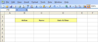
1. Create a New Worksheet (File > New > Blank Worksheet) and add your titles for the Excel table, where the data will be stored.




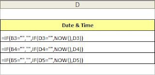
2. In cell D3 (column D, row number 3) you need to enter the following formula
   
   
   =IF(B3="","",IF(D3="",NOW(),D3))
   
   
   This means that IF cell B3 is empty then do not enter a date and time. IF cell B3 is not empty and IF cell D3 is empty, then enter the date and time.
   
   




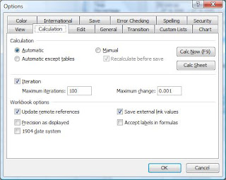
3. Finally, you will need to change the settings within your Excel spreadsheet to stop any Circular References - which is a formula error you get when you try to include your current cell into the formula like we have done here!
   
   
   To remove these errors, select Tools > Options and then select the Calculation tab. Now make sure that the Iteration box is ticked.
   
   




4. And that's all folks!!!
   
   
   Your finished Excel Date Stamp Table should look like this one below, and will record individual dates and times (static dates) for each action.
   

   

Introduction ...

I have spent a lot of time over the years messing around with Microsoft (c) Excel, playing with formulas, and problem solving. A lot of support that I have used to solve my own Excel nightmares have been found within books by authors such as John Walkenbach, and of course the endless online support sites.

* If you are interested in developing your knowledge of Excel, I would highly recommend any of John Walkenbach's books as a valuable learning resource - he is a true Excel guru.

Additionally I have developed my own methods of solving certain Excel based issues, and as time has progressed I have either lost my original notes explaining how I did what I did, or I find that I spend a considerable amount of time finding more and more protracted ways of achieving the same objective.

As it has become more and more time consuming to constantly look-up answers to my questions from a wide range of resources, and collate my own material, I have decided to post my notes, guides, thoughts and resource links within this 'How To Do Excel' blog.

I will endeavour to post regular pieces of information for my own benefit, and for anyone else who wishes to use this blog as a resource tool. Additionally, if you have an Excel question that you need answering then let me know, and I will create a post dedicated to your question.